Snow Mapping With MODIS

Using the MOD10A product from NASA to map snow over time

Snow Mapping

There are many reasons why snow mapping is beneficial. During Spring, we can use it to provide flood risk mitigation — especially for areas prone to flooding. During Winter, it could be used to assess risk for avalanches depending on snowfall and accumulation over time.

Downloading MODIS

download.ipynb

The above script downloads 20 days worth of raw granules over British Columbia. We will be looking at Febuary 5th-25th, 2021. The script contains some functions repurposed from the download script generated from the NSIDC portal. The MODIS snow cover product spatial resolution is 500m x 500m per pixel. This offers a high level view of snow coverage — for more detail, we can use VIIRS (375m x 375x)(VPN10A1.001) or even Sentinel-2 L2A with even further thresholding.

Calculating NDSI Over Time

First we must import our required libraries.

import os

import xarray as xr
import rioxarray as rioxr
import rasterio
import rasterio.plot

import numpy as np
import matplotlib.pyplot as plt

from rioxarray.merge import merge_arrays
from glob import glob

We will consider the bounding box surrounding British Columbia, Canada. The points are lat/long (WSG84 format) since we will be projecting our MODIS data to EPSG4326.

lower_left_lon = -141.899414
lower_left_lat = 47.783635
upper_right_lon = -112.104492
upper_right_lat = 60.866312
bbox = [lower_left_lon, lower_left_lat, upper_right_lon, upper_right_lat]

With our downloaded data, we must first generate our GeoTiffs, cut them to our bounding box and save them as the respective date. We will merge these raw granules that were downloaded using rioxarray by creating a list of open subdatasets. Once merged, we reproject to EPSG4326 and clip to our bounding box AOI

try:
    os.makedirs('mosaic')
except:
    pass
dates = glob(os.path.join('modis','*'))
for date in dates:
    file_pths = glob(os.path.join(date,'*'))
    src_files = []
    for f_pth in file_pths:
        print(f_pth)
        with rioxr.open_rasterio(f_pth) as src:
            src_files.append(src.NDSI_Snow_Cover)
    ds = merge_arrays(src_files)
    ds = ds.rio.reproject('EPSG:4326')
    ds = ds.rio.clip_box(*bbox)
    out_pth = os.path.join('mosaic',f'{os.path.split(date)[-1]}.tif')
    ds.rio.to_raster(out_pth, recale_transform=True)

NDSI

Now we have our mosaics of our AOI, we iterate through them with thresholds to consider if a pixel is snow or not-snow. The snow-cover products document the NDSI values between 0–100, with extra information embedded as values over 200, such as nodata, cloud, missing information/indecision, etc. Since we’re only concerned about the NDSI values, we consider thresholding values above 20 and below 100 inclusive as snow. Anything else will be treated as no-snow. The NDSI value itself if the result of a ratio of the sum and difference of band 4 and band 6 (link):

NDSI = ((band 4-band 6) / (band 4 + band 6))

Though, these products have already had this band math applied and delivered the result, that is the underlying approach.

With each mosaic, we force no-snow pixels to zero and snow pixels to one — this indicates that there was or wasn’t snow in that 500mx500m area that day. Finally, we will then take the mean across all the dates to determine in the last 20 days, how often was that pixel snow covered.

mosaics = glob(os.path.join('mosaic','*'))
ds = xr.Dataset()
for mosaic in mosaics:
    ndsi = rioxr.open_rasterio(mosaic)
    ndsi.data[(ndsi.data > 100)] = 0
    ndsi.data[(ndsi.data < 20)] = 0
    ndsi.data[(ndsi.data != 0)] = 1
    ds[os.path.split(mosaic)[-1]] = ndsi
nds = ds.to_array(dim='mean').mean(dim='mean', skipna=True)
nds.rio.to_raster('mean.tif')

We then can visualize this daily mean with matplotlib and assign a colour map to make it obvious per pixel how often each pixel was covered in snow over the last 20 days.

with rioxr.open_rasterio('mean.tif') as src:
    d = src.data
fig, ax = plt.subplots(1,1,figsize=(20,10))
ax.axis('off')
d[(d==0)] = np.nan
#ax.set_facecolor('k')
im = ax.imshow(d[0], cmap=plt.cm.RdYlBu, vmin=0, vmax=1, clim=[0,1])
fig.colorbar(im, ax=ax)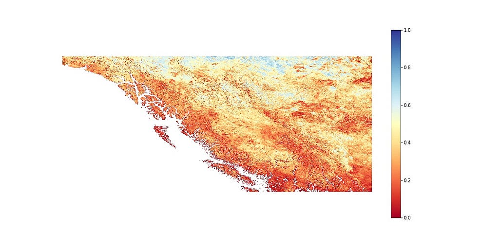

As we can see, it’s no surprise that the northern-most latitude is often snow covered and coastal lines are less so to none. The giant red mass at the bottom left of the mainland is Vancouver, so it’s, again, no surprise that there is not much snow coverage. The rest of the province, depending on the landscape, shows mid-range snow coverage, especially along the mountain ranges.

Github Repository